This textbook was written for the clinical research community at Johns Hopkins leveraging the precision medicine analytics platform (PMAP). These notebooks are available in html form on the Precision Medicine portal as well as in computational form in the CAMP-share folder on Crunchr (Crunchr.pm.jh.edu).

• Platform Tool : Jupyter/Crunchr on PMAP using
• Programming Language : Python 3
• Author(s) : Paul Nagy
• Data access needed to run tutorial on PMAP : CAMP Asthma Database
• License : The notebook is released under the Apache 2.0 License
• Last Updated : May 30th, 2019

Introduction to SQL for mining EMR data

Learning Objectives

1. Introduction on how Electronic Medical Records are organized
2. Learn Structured Querying Language to select records from a database
3. Explore Structured Querying Language for filtering, counting, and grouping of data

Table of contents

• About the table structure of EMR Data
  • Data Schema
  • Key Fields Patient ID & Encounter ID
  • De-identification of patient data
• Introduction to SQL
  • The SELECT statement
  • Using functions (MIN,MAX,COUNT) on columns
  • Filtering columns with WHERE clause
  • Finding distinct values in a column with DISTINCT
  • Filtering data with the WHERE clause
  • Using the IN command to filter by multiple values
  • Filtering by a string with the LIKE command
  • Grouping data with the GROUPBY clause

Working with EMR Data

Clinical patient data is entered into forms of the Epic electronic medical record and converted nightly to a relational database (Clarity). The data is stored in tables of related information. There are currently over 20k tables in the Epic Clarity database.

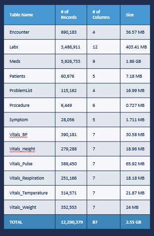
This de-identified dataset contains 60k patients with asthma and pulls commonly used tables as part of clinical care. No narrative fields are included in this dataset. Here is a list of tables that are included in this dataset.

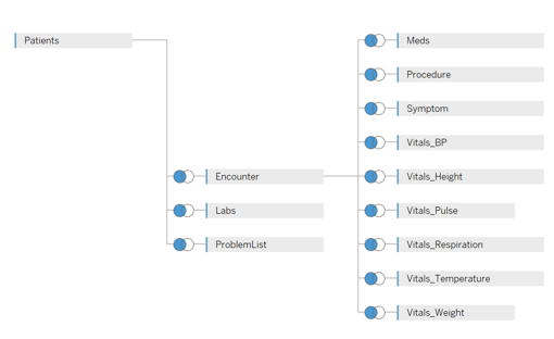
In an EMR, patient records are organized by a patient encounter (such as a office visit or a hospitalization). Each patient may have many encounters, and each encounter may have many observations of vitals as part of each. This relationship (known as an entity relationship) is important for combining many observations around a patient by their encounters.

Import Libraries and Connect to DB

Below are the code cells to connect to the CAMP Asthma database. You can follow along and run the cells or just scroll down to see there pre-compiled output. You will need to enter you JHED to connect to the PMAP database and have requested access for the Asthma dataset.

#Libraries needed
import sqlalchemy
import urllib.parse
import pandas as pd
import getpass
from SciServer import Authentication
myUserName = Authentication.getKeystoneUserWithToken(Authentication.getToken()).userName
passwd = getpass.getpass('Password for ' + myUserName + ': ')
user = "win\\" + myUserName

Password for pnagy2: ········

#SQL Driver
driver="FreeTDS"
tds_ver="8.0"
# Database
host_ip="ESMPMDBPR4.WIN.AD.JHU.EDU" # Update this accordingly
db_port="1433"
db="CAMP_PMCoe_Projection" # Update this accordingly
# Create Connection String
conn_str=("DRIVER={};Server={};PORT={};DATABASE={};UID={};PWD={};TDS_VERSION={}"
.format(driver, host_ip, db_port, db, user, passwd, tds_ver)
)
# Create Engine
engine = sqlalchemy.create_engine('mssql+pyodbc:///?odbc_connect=' +
urllib.parse.quote(conn_str)
)

Database Schema

query="SELECT name, modify_date, max_column_id_used FROM SYS.TABLES;"
data_frame = pd.read_sql_query(query, engine)
table_size=[]
for index,row in data_frame.iterrows():
    #print (row[0])
    tb_name=row[0]
    query="SELECT count(*) as ct FROM [dbo].["+ tb_name + "];"
    df2= pd.read_sql_query(query, engine)   
    table_size.append(df2.ct.loc[0])
data_frame['size']=table_size
data_frame['updated']=data_frame['modify_date'].dt.strftime('%Y/%m/%d')
del data_frame['modify_date']
data_frame.columns=['names','columns','records','updated']
data_frame

	names	columns	records	updated
0	patients	5	60676	2019/05/13
1	encounters	4	753484	2019/05/13
2	labs	12	3509868	2019/05/13
3	meds	10	631022	2019/05/13
4	problemlist	4	781379	2019/05/13
5	procedures	6	5550672	2019/05/13
6	symptoms	5	1967436	2019/05/13
7	vitals_BP	7	1061684	2019/05/13
8	vitals_height	7	305612	2019/05/13
9	vitals_pulse	7	1227099	2019/05/13
10	vitals_respiration	7	957677	2019/05/13
11	vitals_temperature	7	805345	2019/05/13
12	vitals_weight	7	406052	2019/05/13
13	sysdiagrams	5	0	2019/05/09

query="Select COLUMN_NAME,DATA_TYPE FROM INFORMATION_SCHEMA.COLUMNS Where TABLE_NAME='patients'"
df3 = pd.read_sql_query(query, engine)
df3

	COLUMN_NAME	DATA_TYPE
0	osler_id	nvarchar
1	date_of_birth	datetime
2	gender	varchar
3	race	varchar
4	ethnicity	varchar

df3.to_csv('temp.csv')

Structured Query Language Introduction

There is a useful and standard way to ask questions of relational databases known as SQL (Structured Query Language). There are many resources to learn SQL and database querying online based upon the SQL Server database.

SQL is an open standard query language that dates back to the early 1970's to work with databases using relational algebra. It is still the standard for working with relational databases.

• SQL Tutorial
• SQL Cheat Sheet
• SQL Keyword Reference

Here are the basics to querying a database.

SELECT Column_Names FROM Table_Name

The two main elements of querying in SQL are the SELECT statement which specifies which columns to return and the FROM statement which specifies which table to pull those columns from.

query="SELECT TOP 3 * FROM vitals_temperature"
df3 = pd.read_sql_query(query, engine)
df3

	osler_id	encounter_id	encounter_type	admission_date	discharge_date	temperature	temperature_date
0	2dc40218-fbde-482e-8ca5-7cb73a48ec9f	147362	Hospital Encounter	2016-02-14 19:12:00	2016-02-15 17:35:00	98.2	2016-02-15 16:18:00
1	2dc40218-fbde-482e-8ca5-7cb73a48ec9f	147362	Hospital Encounter	2016-02-14 19:12:00	2016-02-15 17:35:00	98.2	2016-02-15 12:18:00
2	2dc40218-fbde-482e-8ca5-7cb73a48ec9f	458661	Hospital Encounter	2016-12-06 16:40:00	2016-12-07 14:45:00	97.3	2016-12-06 20:43:00

In this example we use the * wildcard after the SELECT statement to designate that we want all the columns. We specify vitals_temperature after the FROM statement to specify the temperature table. We send a query string to the database server and it returns the restulst in the form of a table which is stored as a Pandas dataframe df3. Pandas is described in greater detail in upcoming pages. For now focus on the SQL statement.

Try modifying the query string to return only the temperature field and selecting the top 20 records.

Note the Top 3 statement before the * and after the SELECT statement. This specifies that we only want the top 3 records to be returned. the vitals temperature table contains over 314k records and we do not want to return them all for this example.

Select Statement

In this example select the encounter_id and encounter_type columns to be returned as fields.

• SELECT
  • Name of Columns to be included (* for all)
• FROM
  • Which Table(s) to include
• WHERE
  • Conditions to filter row
• GROUP BY
  • Aggregation of results into groups
• HAVING
  • Limits on the aggregated results
• ORDER BY
  • Sort the results

query="SELECT * FROM patients"
df3 = pd.read_sql_query(query, engine)
df3.head(5)

	osler_id	date_of_birth	gender	race	ethnicity
0	5303550b-8ed2-42fd-885a-d32b308b05f3	2013-12-09	Male	Other	Not Hispanic or Latino
1	3ef665bc-8900-4a68-b086-bfbde88d2280	2015-05-27	Male	White or Caucasian	Not Hispanic or Latino
2	39026546-483b-4959-a889-82a4e3bbaa58	1977-03-14	Female	Black or African American	Not Hispanic or Latino
3	dcbd2d5c-2702-4469-988c-ea647963c49a	1970-08-31	Male	White or Caucasian	Not Hispanic or Latino
4	ab7e569a-2224-4540-8054-bcbef6ea0484	2002-02-18	Male	Black or African American	Not Hispanic or Latino

query="SELECT * FROM patients where gender in ('Male','Female')"
df3 = pd.read_sql_query(query, engine)
df3.head(5)

	osler_id	date_of_birth	gender	race	ethnicity
0	5303550b-8ed2-42fd-885a-d32b308b05f3	2013-12-09	Male	Other	Not Hispanic or Latino
1	3ef665bc-8900-4a68-b086-bfbde88d2280	2015-05-27	Male	White or Caucasian	Not Hispanic or Latino
2	39026546-483b-4959-a889-82a4e3bbaa58	1977-03-14	Female	Black or African American	Not Hispanic or Latino
3	dcbd2d5c-2702-4469-988c-ea647963c49a	1970-08-31	Male	White or Caucasian	Not Hispanic or Latino
4	ab7e569a-2224-4540-8054-bcbef6ea0484	2002-02-18	Male	Black or African American	Not Hispanic or Latino

query="SELECT * FROM patients where date_of_birth<'1990-01-01'"
df3 = pd.read_sql_query(query, engine)
df3.head(5)

	osler_id	date_of_birth	gender	race	ethnicity
0	39026546-483b-4959-a889-82a4e3bbaa58	1977-03-14	Female	Black or African American	Not Hispanic or Latino
1	dcbd2d5c-2702-4469-988c-ea647963c49a	1970-08-31	Male	White or Caucasian	Not Hispanic or Latino
2	4047b2fc-df47-4603-b3d0-b325eec83a80	1986-01-20	Female	White or Caucasian	Not Hispanic or Latino
3	2d1ce486-b399-44f6-84e0-0d7e9ddca993	1956-03-21	Female	Asian	Not Hispanic or Latino
4	68c919ee-b719-4120-8a9a-5a5100be07c7	1968-09-30	Female	White or Caucasian	Not Hispanic or Latino

Using functions (min,max,count) on columns

There are several functions that can calculate on an entire column (field0 and return an aggregate result. Let's look at the main demographics table which has a single record for each patient along with their date of birth.

Note: Date of Birth Dates are randomly shifted as part of the de-identification process

query="SELECT count(*),min(date_of_birth),max(date_of_birth) FROM patients"
df3 = pd.read_sql_query(query, engine)
df3

0	60676	1915-06-16	2018-01-31 12:32:00

Finding distinct values in a column with DISTINCT

Getting a distinct list of values from a given column is a great way of performing a quick quality check. Let's check the * of values reported for gender from the demographics table.

query="SELECT distinct gender FROM patients"
df3 = pd.read_sql_query(query, engine)
df3

	gender
0	Unknown
1	Male
2	Female

Filtering columns with WHERE clause

SQL comes with a powerful capability to filter data. In this example we are filtering data from the vitals temperature table by temperature values over 100.

query="SELECT TOP 2 *  FROM vitals_temperature WHERE temperature>100"
df3 = pd.read_sql_query(query, engine)
df3

	osler_id	encounter_id	encounter_type	admission_date	discharge_date	temperature	temperature_date
0	bde80687-7f2c-4f3a-84b6-c0830ed55525	497026	Hospital Encounter	2016-12-14 07:22:00	2016-12-18 19:40:00	101.5	2016-12-16 23:45:00
1	bde80687-7f2c-4f3a-84b6-c0830ed55525	497026	Hospital Encounter	2016-12-14 07:22:00	2016-12-18 19:40:00	102.0	2016-12-17 06:00:00

In this example we filter the type of encounter to Office Visit. Please note the use of double quotations " for the entire SQL string and single quotations for a string match in the WHERE clause. String matching within fields are case sensitive.

query="SELECT TOP 2 * FROM encounters WHERE encounter_type='Office Visit'"
df3 = pd.read_sql_query(query, engine)
df3

	osler_id	encounter_id	encounter_type	encounter_date
0	5303550b-8ed2-42fd-885a-d32b308b05f3	17938	Office Visit	2015-10-10
1	5303550b-8ed2-42fd-885a-d32b308b05f3	142706	Office Visit	2016-01-24

Using the IN command to filter by multiple values

For this example we are going to show how you can enter a multiline string in Python using (). This improves readability.

query=("SELECT TOP 5 * FROM encounters "
       "WHERE encounter_type IN ('Office Visit','Hospital Encounter')")
df3 = pd.read_sql_query(query, engine)
df3

	osler_id	encounter_id	encounter_type	encounter_date
0	5303550b-8ed2-42fd-885a-d32b308b05f3	17938	Office Visit	2015-10-10
1	5303550b-8ed2-42fd-885a-d32b308b05f3	142706	Office Visit	2016-01-24
2	5303550b-8ed2-42fd-885a-d32b308b05f3	571465	Office Visit	2017-03-19
3	5303550b-8ed2-42fd-885a-d32b308b05f3	432470	Office Visit	2016-10-22
4	5303550b-8ed2-42fd-885a-d32b308b05f3	410795	Office Visit	2016-10-01

Filtering by a partial string with the LIKE command

The LIKE function can look through a string field for a pattern match. The % sign indicates there can be any characters before or after the string depending on where you are looking for.

query=("SELECT TOP 3 * FROM meds "
       "WHERE medication_name LIKE '%ALBUTEROL%'")
df3 = pd.read_sql_query(query, engine)
df3

	osler_id	encounter_id	medication_id	order_date	medication_name	dose	therapeutic_class	pharmaceutical_class	pharmaceutical_subclass	extraction_date
0	5303550b-8ed2-42fd-885a-d32b308b05f3	410795	250	2016-10-01	ALBUTEROL SULFATE 2.5 MG/3 ML (0.083 %) SOLUTI...	2.5 mg	ANTIASTHMATICS	BETA-ADRENERGIC AGENTS, INHALED, SHORT ACTING	Asthma/COPD Therapy - Beta 2-Adrenergic Agents...	2018-09-06 16:16:44.973333
1	5303550b-8ed2-42fd-885a-d32b308b05f3	631974	250	2017-05-08	ALBUTEROL SULFATE 2.5 MG/3 ML (0.083 %) SOLUTI...	2.5 mg	ANTIASTHMATICS	BETA-ADRENERGIC AGENTS, INHALED, SHORT ACTING	Asthma/COPD Therapy - Beta 2-Adrenergic Agents...	2018-09-06 16:16:44.973333
2	5303550b-8ed2-42fd-885a-d32b308b05f3	411794	24915	2016-10-03	LEVALBUTEROL 0.63 MG/3 ML SOLUTION FOR NEBULIZ...	.63 mg	ANTIASTHMATICS	BETA-ADRENERGIC AGENTS, INHALED, SHORT ACTING	Asthma/COPD Therapy - Beta 2-Adrenergic Agents...	2018-09-06 16:16:44.973333

Grouping data with the Group By clause

The GROUP BY command groups data by common valued fields. In this example we have a GROUP BY on the type of encounter tied to an aggregate function count. It is important to know that the GROUP BY clause can only be used on columns which also appear in the SELECT statement, and on aggregate functions like COUNT(*) or SUM(). Also note the ORDER BY command which then sorts the resulting data in descending order to show the most frequent encounter *.

query=("SELECT TOP 5 encounter_type,COUNT(*) FROM encounters "
       "GROUP BY encounter_type ORDER BY COUNT(*) DESC")
df3 = pd.read_sql_query(query, engine)
df3

	encounter_type
0	Office Visit	431080
1	Appointment	97718
2	Hospital Encounter	86789
3	Visit Encounter	62740
4	Clinical Support	21626